Reading large datasets for training on Colab
Large datasets on Colab
Google Colab provides a fantastic way for anyone to access a powerful GPU runtime on the cloud, especially tailored for exploring and training machine learning models. However, the issue still remains of making sure the training data that you need is available to your models within a reasonable latency. For small datasets, a common approach is to simply store your data on your local computer, and upload it to the Colab runtime everytime via the internet. This approach is not feasible when datasets become large: in our experience, it can take up to 6 hours to upload a <2 GB dataset to the Colab environment.
We need a faster way to access our training data, possibly by storing it already on the cloud to exploit better bandwidth. We consider three approaches:
- GDrive: using Google Drive for storage, and mounting it in the Colab runtime;
- GCSFuse: using Google Cloud Storage Buckets, and mounting them with gcsfuse;
- GCS Manual: using Google Cloud Storage Buckets, and transferring the data with the storage api.
Main results
The results of this investigation can be summarized as follows:
- the major bottleneck for the performance of reading the training dataset is the time required to transfer the files from their remote location to the Colab environment during the first epoch;
- geographic location plays an important role in affecting the performance, while choosing a cpu, gpu or tpu runtime does not;
- after the first epoch of training, caching the files locally on the Colab runtime significantly improves the performance, to the point that other factors (such as gpu transfers) may become the bottlenecks to training performance.
More specifically, in terms of the performance of the approaches considered here, we found that:
- GCSFuse does not seem to aggressively exploit the read-only nature of ML workflows, meaning that subsequent reads after the first are almost as slow as the first one;
- The GCS Manual approach offers the best performance, but requires payment of a low fee and that you refresh your Colab environment enough times to land in the geographic region that you need;
- GDrive offers good performance for free, but can be a bit unstable when dealing with folders containing lots of files.
Performance analysis
When you create a new Colab runtime, it is attached to an hard drive that does not contain your data. Hence, to access the contents of your files, the data needs to be transferred to the Colab runtime, at least once for every file read. In the third approach described above, this transfer happens when we manually copy the files, but do not be fooled: it happens with the other approaches too, even if it is handled automatically under the hood by the software libraries.
In machine learning workflows, re-reading a file happens very often during training, for example at every epoch. Retransferring the data everytime you want to re-read a file would be costly, so a more efficient strategy is to cache the file contents on the Colab runtime filesystem. This is what’s implicitly happening in the third approach, which works well because you already know that those files have not been changed on the remote server. In the first and second approach you are instead relying on the library’s implementations to handle this cache optimization for you.
To measure the performance of reading files, we use read bandwidth in Megabytes per second. In practice, we measure the amount of MB read and the time it took to read them separately, and plot their ratio. We caution against taking these numbers as an absolute indication of real-world performance, although they are valid to have a ballpark idea. The reason is that other operations, such as opening the file, can contribute significant overhead (especially for small files).
Gcsfuse does not provide optimal re-read performance
We measured the speed of re-reading files for the three approaches described above. While the GCS Manual approach and Google Drive appear to exploit some sort of caching to improve the performance, we observed that gcsfuse’s speed was not improved in subsequent reads of the files. The Figure below shows the boxplots for the file read bandwidth, distinguishing the first transfer from the remote servers versus a second (and subsequent) reads. Note the different scales on the x-axis.
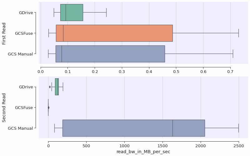
During the first read, all bandwidths are the same. The first read is likely bounded by the speed of transferring the file contents from their cloud locations over the internet. The second read is more than 1000x faster for GDrive and the Manual approach, while for GCSFuse the speed remains roughly the same.
In this benchmark, we did our best to ensure that file contents were not kept in memory between the first and second reads, to simulate the case where one would loop over the whole dataset for each epoch, effectively clearing the memory. It remains unclear why the second-read bandwidth of the GDrive approach is worse than the manual approach, but it might be possible that GDrive is performing some checks or contacting the remote server.
Geographic region affects performance
The closer the remote servers are to where the colab is physically running, the better we expect the performance to be. We measured the first-read bandwidth and found that geographic proximity can give a 2x-10x boost to performance. The Figure below shows the read bandwidth broken down by region where the Colab runtime is executing.
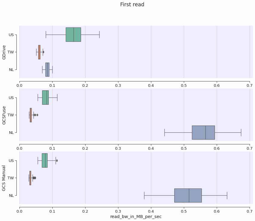
For the GCSFuse and GCS Manual approaches, performance was improved when the colab runtime was running in the Netherlands. This is consistent with the fact that my GCS Bucket is located in the EU Multiregion. The GDrive approach, on the other hand, has better performance when the Colab runtime is in the US. One can only assume that GDrive servers are located there.
Runtime type does not affect performance
As expected, we also confirm that runtime type does not affect first read bandwidth.
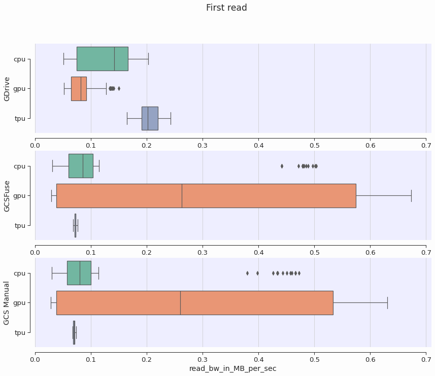
This confirms our understanding that the performance of reading files for the first time is bounded by the time required to transfer the file contents over the internet.
Implementation guide: storing and reading your data from the cloud
This section presents the code and some technical details for implementation.
GDrive: Google Drive for storage and mounting
I used the UI to upload my dataset to my personal Google Drive. Then, the code to mount your drive in the Colab runtime is relatively simple.
from google.colab import drive
drive.mount('/content/gdrive')
Note that calling drive.mount will prompt you for an authorization code, for which you manually need to click on a link.
After authentication and successful mounting, you are able to access all the files on your Google Drive from the Colab runtime.
images = os.listdir('/content/gdrive/path/to/training/data')
with open(path, 'r') as f:
  content = f.readlines()
Google Drive can be a bit clumsy and unstable when dealing with folders containing many files.
An efficient approach to uploading large datasets to Drive is to upload a zipped folder, and unzip it directly on the Drive.
Sometimes, reading the files would fail with an OSError exception or a timeout.
I found that listing the directories containing the training data and catching the exceptions in that moment with the following code can help in later on making the training process more stable.
retry = True
while retry:
  retry=False
  try:
    next(os.walk('/content/gdrive/path/to/training/data'))
  except StopIteration:
    print('Exception Raised. Retry')
    retry = True
GCSFuse: Cloud Storage and gcsfuse
You can use the Google Cloud Storage service to store your dataset. This is a viable option even if you’re not within a corporation or a well-funded research institution, as the prices are not so high. I’ve been storing about 10 GB of data for a couple of datasets, and paying less than 3 EUR per month. A simple way of accessing your data from Colab is then to mount the Storage Bucket on the runtime, using gcsfuse. First, you need to install the tool
!echo "deb http://packages.cloud.google.com/apt gcsfuse-bionic main" > /etc/apt/sources.list.d/gcsfuse.list
!curl https://packages.cloud.google.com/apt/doc/apt-key.gpg | apt-key add -
!apt -qq update
!apt -qq install gcsfuse
Then you need to authenticate yourself and prepare the directory
from google.colab import auth
auth.authenticate_user()
import os
os.makedirs('/content/bucket-data')
os.chdir('/content')
Now you are ready to mount the drive
!gcsfuse --implicit-dirs my_bucket_name bucket-data
The --implicit-dirs option is really important, as it tells gcsfuse to recreate the directory structure from the Cloud Storage Bucket (very important if, for example, train and validation datasets are distinguished by being in different folders).
Note that gcsfuse seems to have some caching options, but when I mounted the drive with the options below I found no significant performance difference
# finer control on caching
!gcsfuse --implicit-dirs --stat-cache-ttl 5h --type-cache-ttl 5h --stat-cache-capacity 65536 ml_datasets_checco_1 bucket-data
After a successful mount, it is again possible to open the files as usual
images = os.listdir('/content/bucket-data/my/path')
with open(path, 'r') as f:
  content = f.readlines()
GCS Manual: Cloud Storage and manual file copy
For performance reasons, we devised a third option in which we copy the files manually from the Storage Bucket using the provided API. Authentication and some preparation is again required
from google.colab import auth
auth.authenticate_user()
import os
if not os.path.exists('/content/gcs-api/my/data'): os.makedirs('/content/gcs-api/my/data')
Then the API can be used to retrieve the files
from google.cloud import storage
client = storage.Client(project='my_project_name')
for bucket in client.list_blobs('my_bucket_name'):
  bucket.download_to_filename('/content/gcs-api/my/data/this_file_name.ext')
As shown above, performance is affected by the region of your GCS Bucket as well as the region where the Colab runtime is executing. The former can be found out through the Google Cloud Console, while the latter can be found using
import requests
ipinfo = requests.get('http://ipinfo.io')
region = ipinfo.json()['country'] + ': ' + ipinfo.json()['region']
Code
The code for the benchmarks can be found here, while the analysis code is here.
We used python’s line profiler %lprun to extract timings for single lines of code.
For GDrive and GCSFuse, the read benchmark looks like this:
N=50
images = os.listdir('/content/gdrive/path/to/data')
for i in range(N):
  filename = images[i]
  path = '/content/gdrive/My Drive/ML_data/snakes/valid/venomous/' + filename
  with open(path, 'rb') as f:
    f.seek(0,2)
    length_of_file = f.tell()
    f.seek(0,0)
    content = f.read(length_of_file)
To obtain the read bandwidth, we divided the total size of the files in MB by the sum of all the timings for the f.read function call, as measured by lprun.
For GCS Manual, the benchmark looks like this:
N=50
i=0
for b in client.list_blobs('gcs_bucket_name'):
  i += 1
  if i >=N:
    break
  filepath = '/content/gcs-api/'+ '/'.join(b.name.split('/')[-4:])
  b.download_to_filename(filepath)
Here we measured instead the time of the b.download_to_filename function.
Technically this doesn’t include reading the file, but once it has been downloaded the file contents can be considered to be in memory, and reading them right away would happen at lightining speed compared to the cost of transferring them from the remote servers.