A Simplified Model for Load Imbalance in Distributed Spiking Neural Networks
Simulating networks of spiking neurons at large scale requires the implementation of some strategy to distribute neurons across different compute nodes. As the network evolves during the simulation some compute nodes may be required, at a given time instant, to process more spikes than other neurons, simply because of the chaotic activity of the network. This introduces a negative effect on simulation performance called load imbalance, by which the total wallclock time of the simulation is increased because some compute nodes must waste cycles waiting for others (who were tasked with a larger amount of computation) to finish.
The load balance problem has been tackled differently in the literature. The developers of NEST, one of the state-of-the-art spiking point-neuron simulators available open-source, have recently stated that “one needs to investigate how to map the spatial structure of a neuronal network to the topology of modern HPC systems. This is not an obvious design choice as the currently employed round-robin distribution scheme is crucial for load balancing. Any non-random distribution of neurons could incur significant performance penalties due to unbalanced work load.” As part of a software engineering effort, the group of Modha et al. have developed a closed-source simulator based on non-blocking communication that is able partially to mitigate the load balancing problem. Finally, a 2014 study from Gerstner’s lab found that synaptic plasticity can greatly impact simulation performance by introducing a significant load imbalance among parallel processes.
In this post, I will introduce a simple model that allows to get an idea of the potential load imbalance that may arise during a simulation under some simplified assumptions.
Results
Under reasonable assumptions, the load imbalance \(\Lambda = max~\{W_p\} - min~\{W_p\}\) arising from the different spiking workloads in a distributed spiking neural network simulation can be estimated by
\[Pr( \Lambda = k ) = \sum_{x=0}^\infty Pr( max~\{W_p\} = x, min~\{W_p\} = x - k ),\]where \(W_p i.i.d.\) and
\[Pr( max~\{W_p\} = x, min~\{W_p\} = y ) = \begin{cases} 0, &x<y \\ [ F_W(y) - F_W(y-1)]^P, &x = y \\ [ F_W(y+1) - F_W(y-1)]^P - [ F_W(y+1) - F_W(y)]^P - [ F_W(y) - F_W(y-1)]^P, & x = y+1\\ [ F_W(x) - F_W(y-1)]^P + [ F_W(x-1) - F_W(y)]^P - [ F_W(x) - F_W(y)]^P - [ F_W(x-1) - F_W(y-1)]^P, &x > y + 1 \end{cases}\]where \(F_W\) is the cdf of \(W_p\).
Application
This result was obtained with the application to the distributed simulation of spiking neural networks in mind. In this case \(W_p\) represents the number of spikes that a given parallel process must integrate in a network minimum delay period. According to the model defined below, \(W_p \sim Poiss( \frac{NK}{P}f\delta)\).
However, the problem is framed in the general setting of finding the distribution of the difference between the maximum and minimum of a collection of i.i.d variables.
Validation
I tested the formula above for \(P=16\) and different values of the Poisson parameter \(\mu\). The numerical experiments yield counts that are very similar to those obtained during the formula.
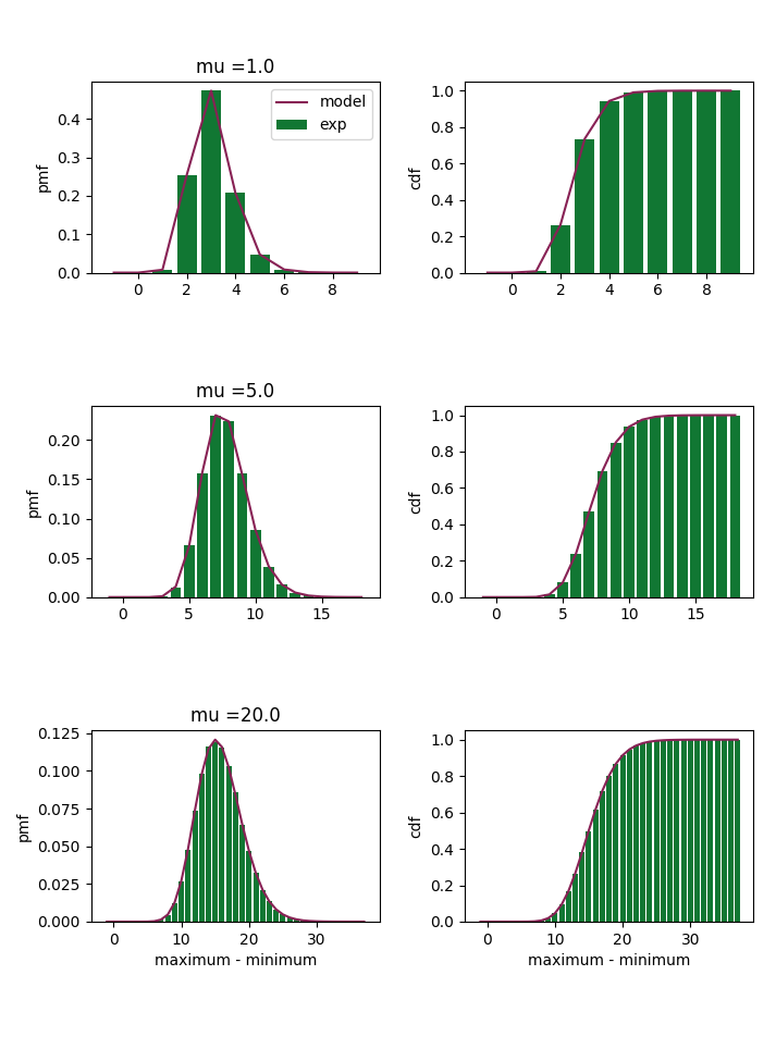
I have observed for \(\mu > 20\) results start being incorrect.
I suspect this may be due to roundoff errors.
This is due to the fact that I approximated the range of values for the sum in the definition of the pmf of \(\Lambda\).
In the new version of the code I have called this variable range_for_convolution and set it to a much larger value.
With a value of range_for_convolution=200., results appear correct at least for \(\mu \leq 100\).
Obviously, this results in a much more computationally expensive process.
In the future, it would be interesting to explore better ways of fixing this problem.
The code for generating this image is provided here.
Problem Definition
As is often done, I will simplify the spiking activity of a neuron and consider it as a poisson process with certain firing rate \(f\). Moreover, I will introduce the simplifying assumption that all neurons are independent from each other. Note that this is a very unrealistic assumption, however it is often done in literature and in any case one may assume that if the neurons are randomly distributed across compute nodes it may still be a valid approximation. Finally, I will assume for simplicity that all neurons have the same firing rate. Again, this is not a very realistic assumption. However this assumption can provide a best-case scenario where the load imbalance originates only from the chaotic and possibly stochastic nature of the spiking neural network, and if we introduce additional imbalance by, for example, having different firing rates than the resulting load imbalance could only get worse.
Let me introduce some notation:
- \(N\) is the total number of neurons in the simulation;
- \(P\) is the number of parallel distributed processes;
- \(f\) is the firing rate of each neuron;
- \(K\) is the number of synapses per neuron;
- \(\delta\) is the interval of simulated time at the end of which we wish to assess the potential load imbalance.
The number of spikes that a neuron must process at a given instant can be modeled by assuming that each of the neuron’s synapses receives events independently from the others and according to a Poisson process as described above. In the case of multisynaptic connections or of small networks this may not be a realistic assumption, but in the case of a large, random network this may be a good approximation.
As a consequence of the assumptions above and assuming that neurons are randomly and evenly distributed across compute nodes, we have the following model.
The number of spikes to be processed by all the neurons pertaining to a given parallel process is distributed like a Poisson variable: \(W \sim Poiss(\frac{NK}{P}f\delta).\)
Moreover, since we want to estimate the load imbalance, we are interested in the difference between the parallel process with the maximum number of spikes to process and the one with the minimum.
We define the load imbalance as \(\Lambda = max~W - min~W\)
where the \(max\) and \(min\) are taken over the different parallel processes.
Probabilistic Setting
We can frame the problem in a general probabilistic setting as:
Given a set of \(P\) i.i.d. variables \(\{W_p\}\), what is the distribution of \(\Lambda = max~\{W_p\} - min~\{W_p\}\)?
This is an interesting problem for two reason: first it requires estimating the joint distribution of the maximum and minimum of a set of i.i.d. variables; second it requires estimating the distribution of the difference of two variables that are not independent.
Marginal Distributions of the Minimum and Maximum
Finding the distribution of the maximum (minimum) of a set of i.i.d. variables is relatively trivial. The idea is to estimate the cumulative distribution function (cdf) of the maximum (minimum) using an insight into the properties of these functions. For the maximum, we have that if the maximum should be smaller than a certain value \(x\), than all the variables in the set should be smaller than \(x\), which translates to \(Pr( max~\{W_p\} \leq x ) = Pr( W_0 \leq x \cap W_1 \leq x \cap \dots )\).
For the minimum, we use some transformations to obtain that \(Pr( min~\{W_p\} \leq y ) = 1 - Pr( W_0 > y \cap W_1 > y \cap \dots )\).
If \(F_W\) is the cdf of \(W\), the insights above lead to
\[\begin{align*} Pr( max~\{W_p\} \leq x ) &= F_W(x)^P, \\ Pr( min~\{W_p\} \leq y ) &= 1 - [ 1 - F_W(y) ]^P. \end{align*}\]Joint Distribution of the Minimum and Maximum
Finding the joint distribution is not so trivial. This stack exchange answer provides the correct path to follow, but contains some typos. These stack exchange answers also provides some insight, but are applied only to special cases. For completeness and correctness, I will repeat the procedure here.
Given a collection of P i.i.d. variables \(\{W_p\}\), we seek the joint distribution of \(( max~\{W_p\}, min~\{W_p\})\).
By drawing a little diagram, you can convince yourself that
\[Pr( max~\{W_p\} \leq x, min~\{W_p\} \leq y ) = Pr( max~\{W_p\} \leq x ) - Pr( max~\{W_p\} \leq x, min~\{W_p\} > y ).\]From the marginals above, we have that \(Pr( max~\{W_p\} \leq x ) = F_W(x)^P\). To estimate the other term, we need to use the same insight as for the marginals: assuming \(y < x\), if the minimum should be larger than \(y\) and the maximum should be less or equal to \(x\), than all the variables in \(\{W_p\}\) should respect this property.
\[\begin{align*} Pr( max~\{W_p\}\leq x, min~\{W_p\} > y ) &= Pr( W_0 > y \cap W_0 \cap \leq x \cap W_1 > y \cap W_1 \cap \leq x \cap \dots ) \\ &= [ F_W(x) - F_W(y) ]^P. \end{align*}\]On the other hand, if \(y \geq x\), then \(Pr( max~\{W_p\}\leq x, min~\{W_p\} > y ) = 0\).
Therefore, we have that
\[Pr( max~\{W_p\} \leq x, min~\{W_p\} \leq y ) = \begin{cases} F_W(x)^P - [ F_W(x) - F_W(y) ]^P, & y < x \\ F_W(x)^P, & y \geq x. \end{cases}\]Joint Probability Mass Function
The stack exchange answer cited above proceeds to compute the pmf directly by differentiation. Given that the variables of interest here are discrete and non-negative, I found that this approach did not work. Instead, I will use the following relationship that is valid for integer, non-negative variables:
\[\begin{align*} Pr(X=x,Y=y) &= Pr( x-1 < X \leq x, y-1 < Y \leq y) \\ &= F_{(X,Y)}(x,y) - F_{(X,Y)}(x-1,y) - F_{(X,Y)}(x,y-1) + F_{(X,Y)}(x-1,y-1) \end{align*}\]After some computations and taking special care of the corner cases we have:
\[Pr( max~\{W_p\} = x, min~\{W_p\} = y ) = \begin{cases} 0, &x<y \\ [ F_W(y) - F_W(y-1)]^P, &x = y \\ [ F_W(y+1) - F_W(y-1)]^P - [ F_W(y+1) - F_W(y)]^P - [ F_W(y) - F_W(y-1)]^P, & x = y+1\\ [ F_W(x) - F_W(y-1)]^P + [ F_W(x-1) - F_W(y)]^P - [ F_W(x) - F_W(y)]^P - [ F_W(x-1) - F_W(y-1)]^P, &x > y + 1 \end{cases}\]Distribution of the Difference
Finally we are ready to compute our quantity of interest. Here, special care must be taken to pick the correct formula for the difference of two non-independent variables. This formula is a special case of the invertible mappings formula (thank you Francesco Casalegno for pointing this out). According to the formula we have
\[Pr( max~\{W_p\} - min~\{W_p\} = k ) = \sum_{x=0}^\infty Pr( max~\{W_p\} = x, min~\{W_p\} = x - k )\]