Pratical Boltzmann Machines
This post collects a couple of tricks that I found useful for implementing, training and debugging Boltzmann Machines. If you’re more interested in the theory, checkout my Boltzmann Machines (BMs) post.
In what follows, I have tried to collect as many doubts as possible among those that came up while implementing a BM (see ).
Everything is so slow
Yes. There doesn’t seem to be much you can do about that. Training BMs is a costly business, and is very slow. And after getting a residence permit in Switzerland, believe me, I know what slow means.
Neuron activations
On the internet I have seen some people use \({0,1}\) as activation values, and others use \({-1,1}\). From the little that I can tell, \({0,1}\) seem to be used more often in practice, whereas \({-1,1}\) appears often in the theoretical presentations. Moreover, \({0,1}\) has a biological interpretation, corresponding to whether the neuron is active/inactive during that stimulus presentation. However, \({-1,1}\) could somehow be related to excitatory/inhibitory neurons. For both approaches all the neuron dynamics, learning rules and so on remain the same, so in the end it shouldn’t make much of a difference. However, who knows if it makes a difference in terms of convergence speed?
Debugging your energy computation
You can reproduce the analytical example from slide 35.
- initialize a Boltzmann machine with 2 visible and 2 hidden units;
- initialize the weight matrix with
and
\[\mathbf{b} = \mathbf{0}\]- reproduce the table in the slide (also in my BM blog post ), computing the energy for every combination of visible and hidden unit values.
See the code under the section “Debugging your energy computation” for a prototypical implementation.
Debugging your sampling/simulated annealing step
You can use the same analytical example from above. In this case, I suggest computing the conditioned probabilities ( e.g. given that \(\mathbf{h} = \left [ 1,1 \right ]^T\) ).
Looking at the relevant rows of the table from slide 35:
| v1 | v2 | h1 | h2 | -Energy | exp( -Energy) | joint probability \(p(\mathbf{v}, \mathbf{h})\) |
|---|---|---|---|---|---|---|
| 1 | 1 | 1 | 1 | 2 | 7.39 | .186 |
| 1 | 0 | 1 | 1 | 1 | 2.72 | .069 |
| 0 | 1 | 1 | 1 | 0 | 1 | .025 |
| 0 | 0 | 1 | 1 | -1 | 0.37 | .009 |
allows us to compute the conditioned partition function
\[Z_{|[1,1]} = 7.39 + 2.72 + 1 + 0.37 = 11.48\]and the conditioned probabilities
| v1 | v2 | conditioned probability |
|---|---|---|
| 1 | 1 | 7.39/11.48 = 0.643 |
| 1 | 0 | 2.72/11.48 = 0.237 |
| 0 | 1 | 1/11.48 = 0.087 |
| 0 | 0 | 0.37/11.48 = 0.032 |
Then you let your MCMC chain run to convergence (i.e. the BM is dreaming) many times, but always clamping the hidden state to \([1,1]\), and you compute a histogram of the outcomes.
In my code you’ll find an implementation of this idea under the section “Test sampling/dreaming procedure”, although I was super lazy and computed the probability of \(v1+v2\) (a scalar) instead of the vector \([v1,v2]\), so that I could use numpy.histogram easily.
A second way to do this is to randomly initialize the network at every time, and making sure that the joint probabilities respect the ones given in the table.
Finally, a third way is to randomly initialize the hidden state to a randomly chosen value, and checking whether the outcome of the dream step respect the marginal probabilities of \(\mathbf{v}\). To be honest, though, I’m not sure if this way is correct, because it sounds like you are making an assumption that the posterior probability of \(\mathbf{h}\) is uniform.
Simulated annealing schedule
Here again I have found some contradictory information on the internet. I have seen both the phrase
as the temperature becomes a very small value
and
as the temperature tends to one.
In the end, the interpretation that I settled on is the following: as the temperature tends to 0, Boltzmann Machines become a deterministic model very similar to Hopfield nets. I don’t think this is generally what you want, so I settled on the idea that the temperature should start at a value \(T_0 >> 1\) and tend to \(T_{end} = 1\).
Keep in mind that if your starting temperature is too large than the first few iterations will be essentially random. This can be useful if you have a large Boltzmann Machine for which the randomly chosen initial value could be very far the steady-state distribution, but can be annoying for small Boltzmann Machines.
Another concept that I struggled with for some time is where the simulated annealing is used: is it “outside” the training loop, or “inside”? In the end, I decided for the following interpretation: simulated annealing is used to help with the optimization process related to inference, and not the gradient descent on the parameters. Therefore, simulated annealing happens every time you do an inference step, i.e. every time you process a new data point or every iteration of the negative phase. In this interpretation, the simulated annealing happens inside the training loop, but outside the Gibbs sampling loop.
A few tips that I found useful are:
- if your input data is rescaled between -1 and 1 and you have a small-medium BM, then a decent starting value for the temperature can be around 20;
- temperature should decrease pretty slowly: I found that making jumps larger than 5 was making convergence harder;
- running about 20-40 Gibbs sampling loops per temperature value turned out to be pretty good for me;
- running at least double the number of Gibbs sampling loops at the final temperature, to make sure everything is stable, seemed to help.
Training
Training has been, in my experience, extremely slow. Learning rates larger than 0.1 seemed to pretty consistently end up exploding the model, and often I ended up using \(\eta = 0.01\) or even \(\eta = 0.005\).
In the code I knew the exact solution so I could compute the error. Convergence was extremely slow:
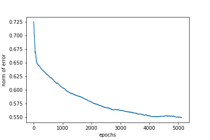
and what’s more, even though the error curve looks pretty promising, the model itself does not yet reproduce the probability distribution in a particularly satisfactory way:
| condition | \(p(\mathbf{v} = [1,1])\) | \(p(\mathbf{v} = [1,0]~or~\mathbf{v} = [0,1] )\) | \(p(\mathbf{v} = [0,0])\) |
|---|---|---|---|
| analytical model \(W_{analytic}\) | 0.15 | 0.48 | 0.37 |
| setting \(W=W_{analytic}\) | 0.16 | 0.47 | 0.37 |
| random initial conditions | 0.29 | 0.51 | 0.2 |
| after convergence | 0.16 | 0.5 | 0.34 |
Discussion
My experience with understanding and training BMs has been somewhat difficult. There is a lot of information on the internet for RBMs, but not so much original BMs. However, the latter are the more biologically realistic, which is ultimately what I was interested in.
I have reached the point where the lowering of my standards due to exhaustion has allowed the current status quo to be sufficient for me to feel satisfied. So overall, a good experience and a Goldmanesque metaphor for life.