A naive explanation of backprop
I got lost trying to implement some simple neural networks from scratch in python. In particular, I figured out that I didn’t really understant how backpropagation works and what is the magic behind it. I decided to inaugurate a blog with my thoughts on backpropagation.
Now, there are many other explanations of backprop out there, much better than mine. Chapter 2 of M. Nielsen’s book is where I learned all this stuff in the beginning. I then went to the deep learning book by Ian Goodfellow, Yoshua Bengio, and Aaron Courville for a deeper but less gentle explanation. Finally, C. Olah’s blog, A. Karpahty’s articles and S. Raval’s hilarious videos all allowed me to get more and more comfortable with different aspects of this problem.
The purpose of this blog post is two fold: first of all, several of the resources above encourage the readers to do the math. This is my attempt at detailing some mathematical expressions, and in turn I encourage everyone to check their calculations against mine and point out any errors/inconsistencies. Second of all, I wanted to get comfortable with the idea of having a blog, and thought this would be a good starting point.
The handwaving backprop explanation
Everyone is talking about it, and everyone has their own, two-sentence explanation that they casually drop in conversation when they want to look cool at a conference. I like to think of myself as a funny guy, so I usually tell the joke:
Backpropagation is merely a rebranding of the chain rule. Yes, I find it quite….. derivative.
if you haven’t fallen off your chair, let me restate what pretty much everybody says about backprop: “in neural networks, the error is associated with the gradient of the cost function. Thanks to the backpropagation algorithm, we have a fast and efficient way of computing this gradient w.r.t every parameter of the model.”
Why Backprop?
Why do we go backwards in the backprop algorithm?
Consider the following simple example.
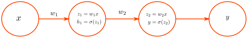
To compute \(y\), we have the following relation:
\[y = \sigma(z) = \sigma( w_2 h_1 ) = \sigma( w_2 \sigma( w_1 x ) ).\]Suppose we want to compute \(\frac{dy}{dw_1}\) and \(\frac{dy}{dw_2}\), applying the chain rule we get:
\[\begin{align*} \frac{dy}{dw_1} & = \frac{d \sigma(z_2) }{dz_2} \frac{ dz_2 }{dw_1 } \\ & = \frac{d \sigma(z_2) }{dz_2} \frac{ dz_2 }{dh_1} \frac{dh_1}{dw_1} \\ & = \frac{d \sigma(z_2) }{dz_2} \frac{ dz_2 }{dh_1} \frac{dh_1}{dz_1} \frac{dz_1}{dw_1} \\ & = \frac{d \sigma(z_2) }{dz_2} w_2 \frac{dh_1}{dz_1} x, \\ \frac{dy}{dw_2} & = \frac{d \sigma(z_2) }{dz_2} \frac{ dz_2 }{dw_2} \\ & = \frac{d \sigma(z_2) }{dz_2} h_1. \end{align*}\]All these formulas look complicated, yet simple enough for our high-school selves to understand them. Isn’t that wonderful!
The trick in backpropagation is noticing that the term \(\frac{d \sigma(z_2) }{dz_2}\) appears several times. First, we need it to compute \(\frac{dy}{dw_2}\). Then, we back-propagate it via \(\frac{d \sigma(z_2) }{dz_2} w_2\) because we also need it to compute \(\frac{dy}{dw_1}\).
The idea is that each layer has the necessary information to compute this error signal, and can pass it backwards to the previous layers which needs it to compute its own derivative (and its own error signals to pass on, if it has previous layers).
Cost function
In the previous example, we wanted to compute the derivative of \(y\). The question arises naturally, \(y\) do you want that? (ah ah).
Well, ideally you have a goal in mind for your network, some sort of cognitive function that you wish it would emulate(e.g. learning to classify handwritten digits from an image). So how do you translate this into some beautiful math that your NN can digest? You postulate the existence of a cost function \(C\). The purpose of a cost function is, in the words of Dr. Evil, to throw us a friggin’ bone. In this simplified point of view, a cost function is a way to massage the neural network’s output in something that is:
- scalar;
- differentiable;
- related to the error in the cognitive function you want to emulate.
So what’s the relationship with learning? The idea is that you are going to tweak and adjust the weights in your network (and generally jump through several hoops) in order to ensure that your neural network does one thing really well: minimize its cost function.
The way you’ll do this is by computing error signals in the form of gradients, and updating network weights accordingly. Therefore you would change the formulas above to compute:
\[\begin{align*} \frac{dC}{dw_1} & =\frac{dC}{dy} \frac{dy}{dw_1}, \\ \frac{dC}{dw_2} & =\frac{dC}{dy} \frac{dy}{dw_2}. \end{align*}\]Why gradients?
This might seem like a pretty silly question, but it still required me some thinking: why exactly do we use the gradient as an error signal?
There are obviously some intuitive explanations for this: as a first approximation, a small change in a parameter corresponds to a change in the output that is proportional to the gradient w.r.t. that parameter. However, the moment of truth that finally put my mind at ease was the realization that using gradients as an error signal is only a consequence of the arbitrary decision of using Gradient Descent as an optimization algorithm. If we were to use different methods (e.g. Newton’s) we would be computing more than just gradients (see e.g. section 8.6 of the deep learning book).
A gentle reminder, the update formula for gradient descent is
\(w_1 \leftarrow w_1 - \eta \frac{dC}{dw_1}\).
We call \(\eta\) the learning rate, a parameter that can have a major effect on convergence.
Scary math in the form of vectors
Let’s take a leap of imagination here and imagine that in the network from the previous example there was at each layer a vector of neurons instead of single ones. I know I’m familiar with this concept, since I applied the same technique at age 14 so I could tell mom I had friends and a girlfriend. Because the devil is in the details, let’s set some dimensions!
\[\mathbf{x} \in \mathbb{R}^{N_{in}},~~~ \mathbf{h}_1 \in \mathbb{R}^{N_1},~~~ \mathbf{h}_2 = \mathbf{y} \in \mathbb{R}^{N_2} .\]Let me state this clearly here, all vectors here are column vectors.
To compute the feedforward part of the neural network, just apply the simple recipe:
\[\begin{align*} \mathbf{z}_1 = & W_1\mathbf{x} \\ \mathbf{h}_1 = & \mathbf{ \sigma } (\mathbf{z}_1) \\ \mathbf{z}_2 = & W_2 \mathbf{h}_1 \\ \mathbf{y} = & \mathbf{ \sigma } (\mathbf{z}_2) \\ cost = & C(\mathbf{y}) \end{align*}\]Now, let me fill you in on some details: \(W_1,W_2\) are matrices whose dimensions are \(N_{this~layer} \times N_{previous~layer}\), i.e.:\(W_1 \in \mathbb{R}^{ N_1 \times N_{in} }, W_2 \in \mathbb{R}^{ N_2 \times N_1 }.\) The function \(\mathbf{ \sigma}\) transforms a vector into another vector with same dimensions \(\mathbf{ \sigma}: \mathbb{R}^N \to \mathbb{R}^N\) whereas \(C\) transforms a vector into a scalar \(C: \mathbb{R}^{N_2} \to \mathbb{R}\).
How do we rewrite the gradient descent formula for vectors? Easy, just look at it component-wise:
\[w_{1,ij} \leftarrow w_{1,ij} + \frac{dC}{dw_{1,ij}}.\]Now, evaluating the derivative requires some math-fu. We start by writing the feedforward relationship component-wise:
\[\begin{align*} y_u & = \sigma( z_{2,u} ) \\ & = \sigma \left ( \sum\limits_m^{N_1} w_{2,um}h_{1,m} \right ) \\ & = \sigma \left ( \sum\limits_m^{N_1} w_{2,um} \sigma \left ( \sum\limits_{p}^{N_{in}} w_{1,mp}x_p \right ) \right ) \end{align*}\]so we can write:
\[\begin{align*} \frac{dC}{dw_{1,ij}} & = \sum\limits_u^{N_2} \frac{dC}{dy} \Bigg|_{y_u} \frac{dy_u}{dw_{1,ij}} \\ & = \sum\limits_u^{N_2} \frac{dC}{dy} \Bigg|_{y_u} \frac{ d\sigma }{dz} \Bigg|_{z_{2,u}} \frac{d z_{2,u} }{dw_{1,ij}} \\ & = \sum\limits_u^{N_2} \frac{dC}{dy} \Bigg|_{y_u} \frac{ d\sigma }{dz} \Bigg|_{z_{2,u}} \left [ \sum\limits_m^{N_1} w_{2,um} \frac{ d h_{1,m} }{dw_{1,ij}} \right ] \\ & = \sum\limits_u^{N_2} \frac{dC}{dy} \Bigg|_{y_u} \frac{ d\sigma }{dz} \Bigg|_{z_{2,u}} \left [ \sum\limits_m^{N_1} w_{2,um} \frac{ d\sigma }{dz} \Bigg|_{ z_{1,m} } \left ( \frac{d}{dw_{1,ij}} \sum\limits_{p}^{N_{in}} w_{1,mp}x_p \right ) \right ]. \end{align*}\]And now we simplify:
\[\frac{d}{dw_{1,ij}} \sum\limits_{p}^{N_{in}} w_{1,mp}x_p = \begin{cases} x_j & \text{if } m = i\\ 0 & \text{otherwise}, \end{cases}\]and we are left with
\[\frac{dC}{dw_{1,ij}} = \sum\limits_u^{N_2} \frac{dC}{dy} \Bigg|_{y_u} \frac{ d\sigma }{dz} \Bigg|_{z_{2,u}} w_{2,ui} \frac{ d\sigma }{dz} \Bigg|_{ z_{1,i} } x_j.\]Now we’re gonna be fancy and write this back into matrix notation. We’re going to use this rule
\[\sum\limits_u k_ua_{ui} \to \text{the } i^{th} \text{ component of } A^T\mathbf{k},\]and introduce the outer product \(\otimes\) between \(\mathbf{x} \in \mathbb{R}^{N_x}\) and \(\mathbf{y} \in \mathbb{R}^{N_y}\) such that
\[\begin{align*} & \mathbf{x} \otimes \mathbf{y} \in \mathbb{R}^{N_x \times N_y} \\ & \left [ \mathbf{x} \otimes \mathbf{y} \right ]_{ij} = x_iy_j, \end{align*}\]and introduce also the simpler element-wise product \(\left [ \mathbf{x} \odot \mathbf{y} \right ]_i = x_iy_i\).
We can finally say that \(\frac{dC}{dw_{1,ij}}\) will be the \((ij)^{th}\) component of the matrix
\[\left [ W_2^T \left ( \nabla C \Bigg|_{\mathbf{y}} \odot \frac{ d \sigma }{dz} \Bigg|_{\mathbf{z}_{2}} \right ) \right ] \odot \frac{ d \sigma }{dz} \Bigg|_{\mathbf{z}_{1}} \otimes \mathbf{x}.\]By repeating the exact same computations, but simpler, we can get the expression for \(\frac{dC}{dw_{2,ij}}\) as the \((ij)^{th}\) component of the matrix
\[\left ( \nabla C \Bigg|_{\mathbf{y}} \odot \frac{ d \sigma }{dz} \Bigg|_{\mathbf{z}_{2}} \right ) \otimes \mathbf{h}_1.\]As a validation, you can check that the above formula is indeed an \((N_2 \times N_1)\) matrix.
The backprop insight
This is where the magic happens! We can summarize our gradient descent formulas as
\[\begin{align*} W_2 \leftarrow & W_2 - \eta \left ( \nabla C \Bigg|_{\mathbf{y}} \odot \frac{ d \sigma }{dz} \Bigg|_{\mathbf{z}_{2}} \right ) \otimes \mathbf{h}_1 \\ W_1 \leftarrow & W_1 - \eta \left [ W_2^T \left ( \nabla C \Bigg|_{\mathbf{y}} \odot \frac{ d \sigma }{dz} \Bigg|_{\mathbf{z}_{2}} \right ) \right ] \odot \frac{ d \sigma }{ dz} \Bigg|_{\mathbf{z}_{1}} \otimes \mathbf{x}. \end{align*}\]As we noted before, one term is repeated in the two expressions, namely \(\left ( \nabla C \Bigg|_{\mathbf{y}} \odot \frac{ d \sigma }{dz} \Bigg|_{\mathbf{z}_{2}} \right )\). Moreover, this repeated term can be computed using only knowledge from the cost function and layer 2. We can use this insight to define an error signal that gets backpropagated through the network.
We are left with the following backprop algorithm:
- compute the gradient of the cost function, evaluated on the activations of the last layer;
- set the error signal \(\mathbf{ \delta } = \nabla C \Bigg|_{\mathbf{y}}\)
- for each layer \(l\) going backwards:
- update the weight matrix \(W_l \leftarrow W_l - \eta \left ( \mathbf { \delta } \odot \frac{ d \sigma }{dz} \Bigg|_{\mathbf{z}_{l}} \right ) \otimes \mathbf{h}_{l-1}\);
- backpropagate the error signal \(\mathbf { \delta } = W_l^T \left ( \mathbf { \delta } \odot \frac{ d \sigma }{dz} \Bigg|_{\mathbf{z}_{l}} \right )\).
Show me the code!
A simple implementation that pretty much follows the notation from this blog post is here.